Pie chart map with displacement and leader lines

Draws a pie chart at each station on a map. When pies would overlap in crowded regions, the pies are displaced asymmetrically away from their true station coordinates and a leader line + anchor dot is drawn so the viewer can still tell which pie belongs to which station. Works with any grouping (phytoplankton groups, zooplankton orders, microbial phyla, ...) and any numeric value (biomass, biovolume, abundance, ...).

Usage

create_pie_map(
  data,
  station_col = "station_name",
  lon_col = "sample_longitude_dd",
  lat_col = "sample_latitude_dd",
  group_col = "group",
  value_col = "value",
  label_col = station_col,
  group_levels = NULL,
  group_colors = NULL,
  group_labels = NULL,
  radius = 0.28,
  size_by = NULL,
  size_range = c(0.15, 0.4),
  repel = TRUE,
  min_sep = 2.4,
  min_disp = 1.6,
  show_labels = TRUE,
  label_size = 3,
  pie_border_color = "white",
  pie_border_width = 0.3,
  leader_color = "gray20",
  leader_width = 0.5,
  anchor_color = "gray10",
  anchor_fill = "white",
  anchor_size = 1.8,
  basemap = NULL,
  basemap_source = c("ne", "eea", "obis"),
  basemap_scale = "medium",
  basemap_fill = "gray95",
  basemap_border = "gray70",
  sea_color = "aliceblue",
  xlim = NULL,
  ylim = NULL,
  pad = 1,
  title = NULL,
  legend_title = "Group",
  verbose = TRUE
)

Arguments

data

A long-format data.frame with one row per (station, group). Required columns are configurable through the *_col arguments and default to station, lon, lat, group, value.

station_col, lon_col, lat_col, group_col, value_col

Column names in data. Defaults match SHARK conventions: "station_name", "sample_longitude_dd", "sample_latitude_dd", "group", "value".

label_col

Column to use for the on-map station label. Defaults to station_col. Set to NULL (and show_labels = FALSE) to omit labels entirely.

group_levels

Optional character vector controlling the legend and slice ordering. Groups not present in data are dropped.

group_colors

Optional named character vector of colors, keyed by group name. If NULL, ggplot's default discrete palette is used.

group_labels

Optional named character vector of legend labels, keyed by group name. Labels may include HTML markup (requires the ggtext package to render).

radius

Pie radius in latitude degrees. Default 0.28.

size_by

Optional. NULL (default) draws all pies at radius. "total" scales each pie's radius by the square root of the station's total value. Any other character value is interpreted as the name of a numeric per-station column in data (e.g. chlorophyll, secchi depth); values are averaged per station when duplicated across rows.

size_range

Numeric length-2: minimum and maximum radius (in latitude degrees) when size_by is set. Default c(0.15, 0.40).

repel

Logical. Run the displacement algorithm? Default TRUE.

min_sep

Minimum center-to-center separation between two pies, expressed as a multiple of the larger of the two radii. Default 2.40.

min_disp

Minimum displacement for a pie that has been moved at all, as a multiple of its radius. Default 1.60.

show_labels

Logical. Draw station labels next to each pie?

label_size

ggplot text size for the station labels.

pie_border_color, pie_border_width

Aesthetics for the slice borders.

leader_color, leader_width

Aesthetics for the leader segments drawn from anchor to displaced pie edge.

anchor_color, anchor_fill, anchor_size

Aesthetics for the dot drawn at the true station location of each displaced pie.

basemap

Optional ggplot layer (or list of layers) used as the base map. If NULL, a coastline polygon from the source named by basemap_source is drawn.

basemap_source

One of "ne" (Natural Earth, default), "eea", or "obis". Ignored when basemap is supplied.

"ne" uses rnaturalearth::ne_countries() (requires the rnaturalearth package).
"eea" uses the high-resolution European Environment Agency coastline (Europe only).
"obis" uses the global OBIS land polygon. For "eea" and "obis" the polygon dataset is downloaded once and cached on disk.

basemap_scale

Resolution passed to rnaturalearth::ne_countries() when basemap is NULL and basemap_source = "ne". One of "small", "medium" or "large". Ignored for the eea and obis sources.

basemap_fill, basemap_border, sea_color

Colors for the default coastline basemap.

xlim, ylim

Optional numeric length-2 vectors. If supplied they override the auto-fitted map extent.

pad

Padding (in degrees) added around station bounds when auto-fitting the extent.

title, legend_title

Optional plot title and legend title.

verbose

Logical. If TRUE (default) print progress messages when a coastline dataset has to be downloaded (only triggered by basemap_source = "eea" or "obis" on the first call). Set to FALSE to keep examples / pkgdown output clean.

Value

A ggplot object.

Details

Coastline sources available via basemap_source when basemap = NULL:

"ne" - Natural Earth 1:10m / 1:50m / 1:110m land vectors, fetched on the fly through rnaturalearth::ne_countries(). Resolution is controlled by basemap_scale. See https://www.naturalearthdata.com. Requires the rnaturalearth and rnaturalearthdata packages (both Suggests).
"eea" - high-resolution European coastline from the European Environment Agency (EEA Coastline 2017). Best choice for detailed regional maps of European waters. Downloaded chunked from the EEA arcgis service the first time and cached locally. Dataset metadata: https://sdi.eea.europa.eu/catalogue/datahub/api/records/9faa6ea1-372a-4826-a3c7-fb5b05e31c52/formatters/xsl-view?output=pdf&language=eng&approved=true.
"obis" - global land polygon distributed by the Ocean Biodiversity Information System, downloaded from https://obis-resources.s3.amazonaws.com/land.gpkg.

The "eea" and "obis" datasets are cached across sessions and can be cleared with clean_shark4r_cache().

Examples

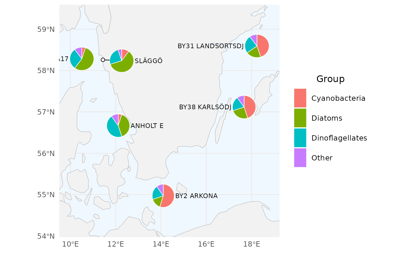
# Six SHARK monitoring stations spanning the Swedish west coast,
# Kattegat, and Baltic Proper. Note that SLÄGGÖ and Å17 sit close
# enough on the Skagerrak shelf that their pies will be repelled and
# drawn with leader lines.
stations <- dplyr::tibble(
  station_name = rep(c("SLÄGGÖ", "Å17", "ANHOLT E", "BY2 ARKONA",
                       "BY31 LANDSORTSDJ", "BY38 KARLSÖDJ"), each = 4),
  sample_latitude_dd  = rep(c(58.25984, 58.28434, 56.66866, 54.97116,
                              58.59366, 57.11717), each = 4),
  sample_longitude_dd = rep(c(11.43567, 10.50432, 12.11117, 14.09883,
                              18.23633, 17.66867), each = 4),
  group = rep(c("Diatoms", "Dinoflagellates",
                "Cyanobacteria", "Other"), 6),
  value = c( 60, 25, 10,  5,   # SLÄGGÖ
             55, 30,  5, 10,   # Å17
             40, 45,  5, 10,   # ANHOLT E
             15, 20, 55, 10,   # BY2 ARKONA
             20, 25, 45, 10,   # BY31 LANDSORTSDJ
             25, 20, 45, 10)   # BY38 KARLSÖDJ
)

# The default basemap uses `rnaturalearth` + `rnaturalearthdata` (both
# Suggests); each example below is guarded by a single-line check so the
# plots render inline rather than all at once after a large `if` block.
has_basemap <- requireNamespace("rnaturalearth",     quietly = TRUE) &&
               requireNamespace("rnaturalearthdata", quietly = TRUE)

# \donttest{
# 1. Uniform pie size, default palette, automatic map extent.
if (has_basemap) create_pie_map(stations)


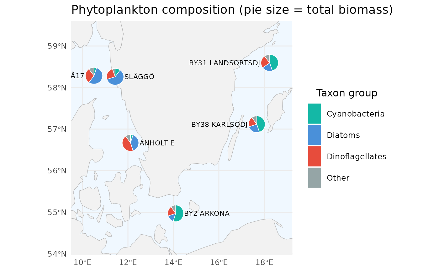
# 2. Scale pie radius by the station's total value (`size_by = "total"`):
#    stations with larger summed biomass get bigger pies. `size_range`
#    controls the smallest/largest radius (in latitude degrees). Pie
#    sizes are relative within the plot only; no size legend is drawn.
if (has_basemap) create_pie_map(
  stations,
  size_by      = "total",
  size_range   = c(0.20, 0.55),
  group_colors = c(Diatoms         = "#4A90D9",
                   Dinoflagellates = "#E74C3C",
                   Cyanobacteria   = "#14B8A6",
                   Other           = "#95A5A6"),
  legend_title = "Taxon group",
  title        = "Phytoplankton composition (pie size = total biomass)"
)


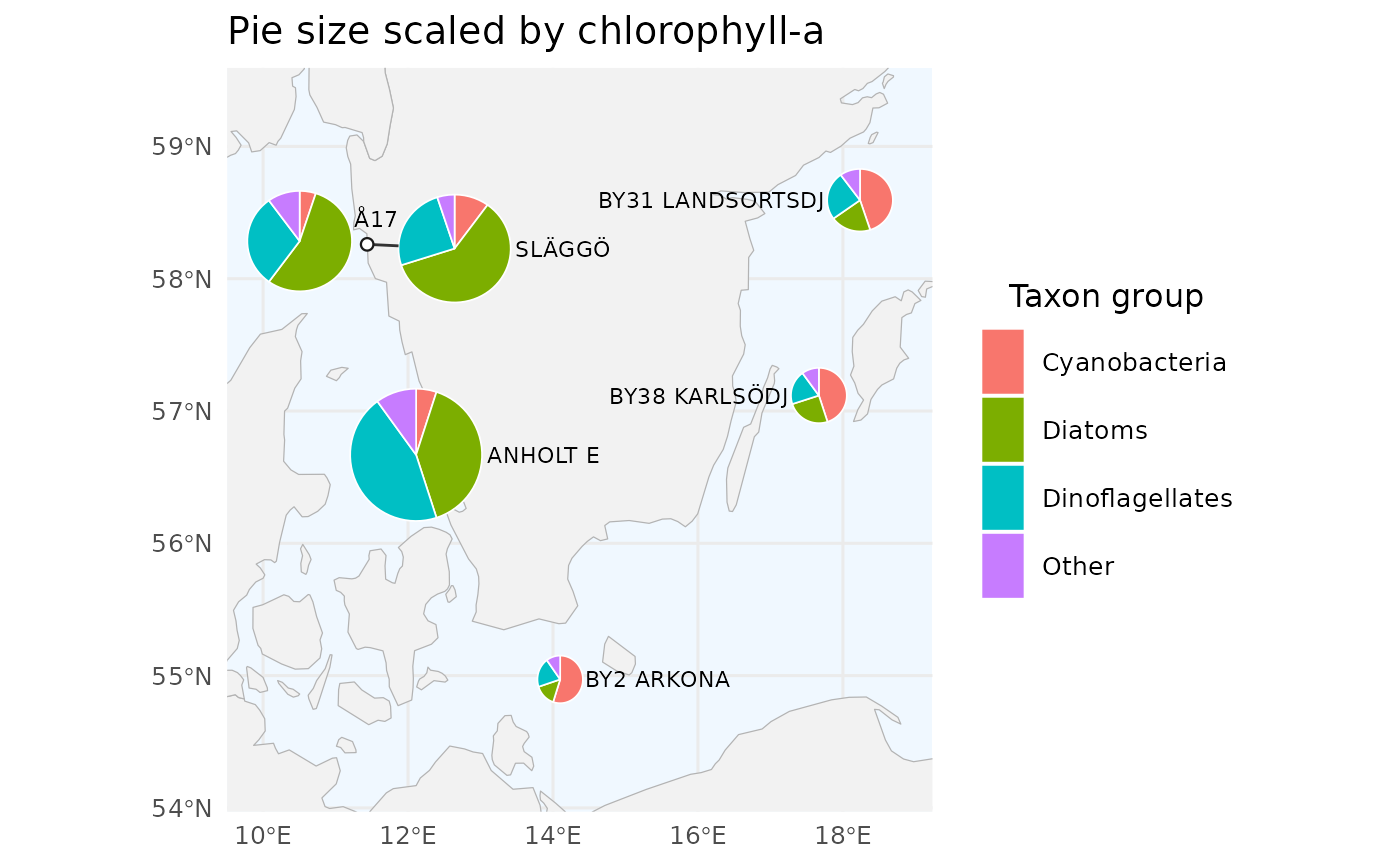
# 3. Scale pie radius by an external per-station metric. Here we add a
#    fake chlorophyll-a column and pass its name to `size_by` - any
#    numeric per-station column in `data` works (e.g. secchi depth,
#    cell counts, nutrient concentrations).
stations$chla <- rep(c(3.1, 2.8, 4.2, 1.1, 1.5, 1.3), each = 4)
if (has_basemap) create_pie_map(
  stations,
  size_by      = "chla",
  size_range   = c(0.18, 0.50),
  legend_title = "Taxon group",
  title        = "Pie size scaled by chlorophyll-a"
)


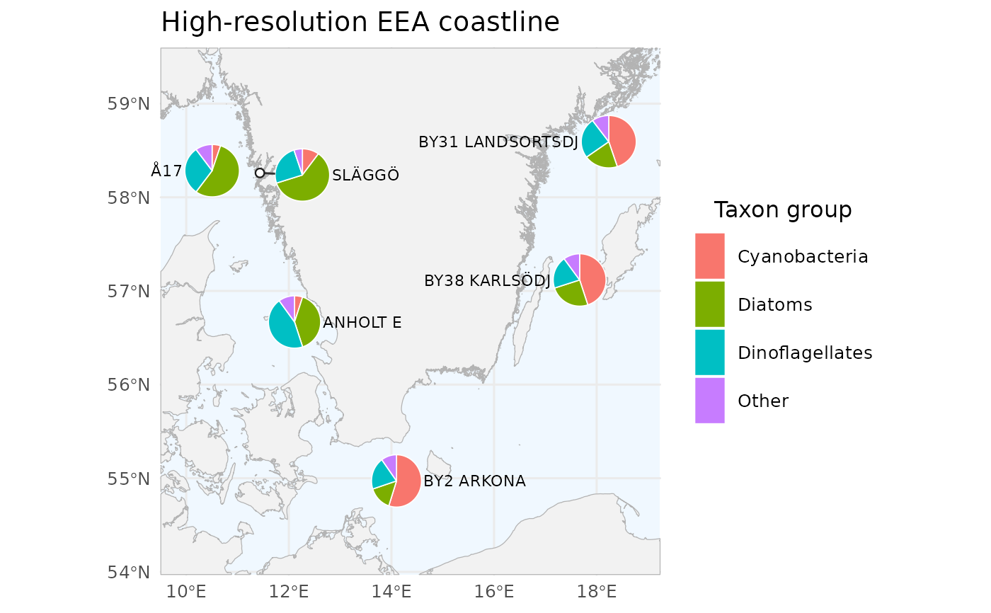
# 4. Use the high-resolution EEA coastline instead of the Natural Earth
#    default. The first call downloads the EEA polygon and caches it
#    for re-use; subsequent calls are fast. `basemap_scale` is ignored
#    for EEA. Suitable for regional European maps where Natural Earth's
#    coastline is too coarse.
try(create_pie_map(
  stations,
  basemap_source = "eea",
  legend_title   = "Taxon group",
  title          = "High-resolution EEA coastline",
  verbose        = FALSE
))

# }